CS180 Project 5

Part 0 – Prompting and Sampling

To demonstrate the usage of the DeepFloyd IF diffusion model, below are a few examples of different prompts using 20 inference steps with stage 1 of the model, which generates images at 64x64 resolution. Using a seed value of 180:

Images generated with num_inference_steps=20

Prompt 1 – 'a photo of a hipster barista'

Using stage 2, we can take the output of stage 1 and upscale it to 256x256 resolution:

By increasing the inference steps, we can generate higher quality images at the cost of more compute time. Below are the stage 2 outputs with the number of inference steps at 100:

Images generated with num_inference_steps=100

From the above, we can see that with longer prompts, we can generate images with more specific details.

Part 1.1 – The forward process

To start, we have the original Campanile image at 64px:

To add noise to an image x₀, we can use the forward process and compute

for a given timestamp t ∈ [0, 1, ..., 999, 1000]. The noise coefficient at timestamp t can be obtained using

alphas_cumprod = stage_1.scheduler.alphas_cumprod
alpha_cumprod_t = alphas_cumprod[t]

for a given t. Below are examples of the Campanile at noise timestamps 250, 500, and 750:

Campanile at Different Noise Levels

Part 1.2 – Classical Denoising

In order to try to revert the image with noise, we can attempt the classical method for denoising. Namely, Gaussian filtering. However, with high noise, the effect is limited:

Noisy vs Gaussian-Denoised Campanile

Part 1.3 – Implementing One Step Denoising

A more effective method is to use a pretrained diffusion model. Using stage_1.unet, we can estimate the amount of noise in the noisy image. With the forward process defined above, we can solve for x₀ (the original image) given x_t (the noisy image) at timestamp t:

at_x0 = im_noisy_cpu - (1 - alpha_cumprod).sqrt() * noise_est
original_im = at_x0 / alpha_cumprod.sqrt()

This method of estimating the clean image given a noisy image is known as one-step denoising. Below is a comparison of the original, noisy, and the estimate of the original image for t ∈ [250, 500, 750]:

Original, Noisy, One-Step Estimate (t = 250, 500, 750)

t = 250

t = 500

t = 750

Part 1.4 – Iterative Denoising

Instead of using one-step, we can obtain better results by iteratively denoising from step t until step 0. However, this means running the diffusion model 1000 times in the worst case, which is slow and costly. Fortunately, we can speed up the computation by first defining a series of strided timestamps, starting at close to 1000 and ending at 0. For the examples below, we will use strided_timestamps = [990, 960, ..., 30, 0]. Then, we can use the formula

to compute x at timestamp T, where T (or prev_t) is the next timestamp after the current timestamp in the strided timestamps. First, we use the definition of the constants, where alpha_cumprod_t is the variable with the bar:

alpha_cumprod_t = alphas_cumprod[t]
alpha_cumprod_prev = alphas_cumprod[prev_t]
alpha_t = alpha_cumprod_t / alpha_cumprod_prev
beta_t = 1 - alpha_t

Then, we can get an approximation of x₀ by using the one-step estimate. The estimated variance will be computed along with the noise estimate, allowing us to calculate x_T using the formula above and obtain the image estimate for the next step. Below are some visualizations for the iterative denoising process:

Denoising Loop Visualizations (i_start = 10)

Noisy Campanile at `t = strided_timestamps[i_start]` (t = 690):

The iterative denoising loop

Final predicted clean images

As we can see, the iterative denoising process produced a more detailed image.

Part 1.5 – Diffusion Model Sampling

Starting with pure noise, we can obtain random denoise images by setting the starting index of strided_timestamps to 0, and using the prompt 'a high quality photo'. Below are a few examples:

Part 1.6 – Classifier-Free Guidance (CFG)

To improve the quality of the images, we can compute both a noise estimate conditioned on the text prompt and the unconditional noise estimate based on the null prompt ''. Denoting the conditional noise estimate as ε_c and the unconditional noise estimate as ε_u, we let our noise estimate be ε = ε_u + γ(ε_c - ε_u). Note that we have ε = ε_u and ε = ε_c for γ = 0 and γ = 1 respectively. However, when γ > 1, we can get much higher equality images for reasons still discussed today. This technique is known as classifier-free guidance. By using γ = 7 and the conditional & unconditional prompts be 'a high quality photo' & the null prompt '', we get the following sample images:

These settings (γ = 7 and the unconditional prompt being '') will be used in all future usage of the CFG iterative denoise function.

Part 1.7 – Image-to-image Translation

Similar to how we added noise to an existing image before denoising the result in part 1.4, we can use the iterative_denoise_cfg function to get a result that is of higher quality, as opposed to merely a prediction of the original. By adjusting the starting amount of noise to the Campanile with the timestamp index i_start, where a higher index means less noise, we get a series of edits that gradually go from entirely new to resembling the original image:

Edits of the Campanile (Noise Levels [1, 3, 5, 7, 10, 20])

Below are 2 other examples of editing similar images:

Test Image 1 (Eiffel Tower)

Test Image 2 (St. Basil's Cathedral)

1.7.1 – Editing Hand-Drawn and Web Images

The same procedure can also be done for images that are hand-drawn or non-realistic:

Web Image (magic gauntlet from gdbrowser.com)

Hand Drawn Image 1

Hand Drawn Image 2

1.7.2 – Inpainting

Using the techniques above, we can also modify our iterative_denoise_cfg function to edit certain sections of an image. To do so, we first define a mask the same size as the image that is 1 at the pixels where we want to edit, and 0 otherwise. For each loop of the denoising process, we replace x_t with mx_t + (1 - m)forward(x₀, t), where m is the mask and x₀ is the original image.

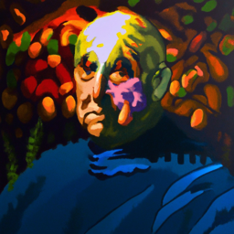
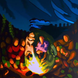
Once image is replaced by masked_image, we replace all further occurrences of image except for the last instance, as the image at each step still needs to be updated. Finally, we let our starting noise be purely random and start with a timestamp index of 0, so that the patch we want to change can be sufficiently denoised. Below are the results on the Campanile image:

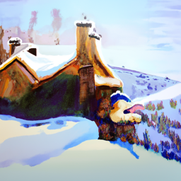
Campanile Inpainting

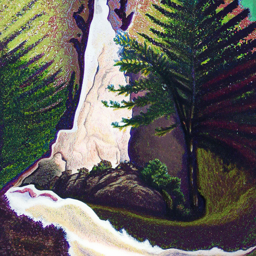
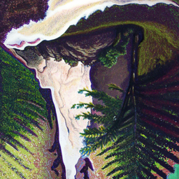
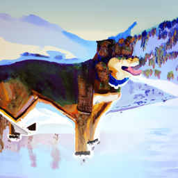
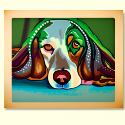
Below are 2 other examples of inpainting similar images:

Eiffel Tower Inpainting

St. Basil's Cathedral Inpainting

1.7.3 – Text-Conditioned Image-to-image Translation

Finally, we can also change our conditional prompt, namely 'a high quality photo', to any other. This will give control over what the noise is projected to, resulting in a series of images that look more like the original image, but also similar to the conditional prompt.

Campanile with prompt `'a pencil'`

Eiffel Tower with prompt `'a rocket ship'`

St. Basil's Cathedral with prompt `'an oil painting of a snowy mountain village'`

Part 1.8 – Visual Anagrams

We now have the necessary tools to generate visual anagrams, or images that look like another different one when flipped/rotated. As an example for a vertical flip anagram, we would start with 2 prompt embeddings p₁ and p₂. For p₁, we would compute the noise estimate ε₁ normally at each step, but for p₂, we flip the image x_t first before computing the noise estimate, then flip back the estimate to obtain ε₂, which would be the noise estimate of the flipped image.

Once this is done, we will use the average of ε₁ and ε₂ as the final noise estimate for each step. The variance can also be computed similarly, namely v₁ will be computed in the usual way, while v₂ will be the flipped variance estimate of the flipped x_t, and the final variance estimate will (v₁ + v₂) / 2. Below are a few examples of such an effect, with p₁ being the first prompt and p₂ being the second:

Prompts: `'an oil painting of an old man'` & `'an oil painting of people around a campfire'`

Prompts: `'a lithograph of waterfalls'` & `'a man wearing a hat'`

Prompts: `'an oil painting of a snowy mountain village'` & `'a photo of a dog'`

Part 1.9 – Hybrid Images

With the techniques above, we can now also create hybrid images, or images that look like different subjects depending on the viewing distance. The classical way to create a hybrid image is to transform the image you want to see at a far range with a low-pass filter, the image you want to see at close range with a high-pass filter, and combine the 2 transformed images. We can use a similar algorithm in the denoising process, namely by passing the noise estimate from p₁ and p₂ through a low and high pass filter, respectively.

After doing so, we will add the 2 filtered noises together to get the final noise estimate at each step. This will produce an image that, when viewed close up, shows p₁, but when viewed far away, shows p₂. Unlike the anagram images, we don't need to flip or transform the image to be denoised, as both images should be viewed under the same orientation. Below are several examples:

Prompts: `'a lithograph of a skull'` (low-pass) & `'a lithograph of waterfalls'` (high-pass)

Prompts: `'a pencil'` (low-pass) & `'a rocket ship'` (high-pass)

Prompts: `'a lithograph of waterfalls'` (low-pass) & `'a photo of a dog'` (high-pass)

Part 2 – Implementing the UNet from scratch

Now that we know how we can generate images with the help of a UNet in a denoising model, we will go through implementing one from scratch. More specifically, we will be attempting to generate digits similar to those in the MNIST dataset from pure noise using a denoising UNet that we will create.

Training an Unconditioned UNet

The most basic denoiser is a one-step denoiser. Formally, given a noisy image z, we aim to train a denoiser D_θ(z) that can map it to a clean image x. To do this, we can optimize over the L² loss E_z,x||D_θ(z)||² while training.

To create a noisy image, we can use the process z = x + σε where σ ∈ [0, 1] and ε ~ 𝒩(0, 𝐈). Here, 𝒩 is the standard normal distribution. To visualize the kind of images this process will result in, below is an example of an MNIST digit with progressively more noise as σ gradually increases from 0 to 1:

To start building the model, we will be using the following architecture:

where D is the number of hidden dimensions.

Training hyperparameters

For the hyperparameters, we will be using a batch size of 256, a learning rate of 1e-4, a hidden dimension of 128, the Adam optimizer with the given learning rate, and a training time of 5 epochs. A fixed noise level of σ = 0.5 will be used to noise the training images.

Evaluation results

After the model is trained, below is the training loss curve, where the loss of the model is plotted for every batch processed:

The following are the performance of the model after the 1st and 5th epoch on sample test images, all noised with σ = 0.5:

We can see that the model performs decently on different digits. To illustrate its effectiveness on images noised with different levels of σ below is the model after the 5th epoch denoising the same image with different levels of noise for σ ∈ [0.0, 0.2, 0.4, 0.5, 0.6, 0.8, 1.0]:

Although the model works well for images with small amounts of noise, the more noise the image has, the less quality of the model's prediction.

Limitations on pure noise

Although the model is decent at removing noise from images, our goal is to generate digits from pure noise. This proves to be an issue because with MSE loss, the model will learn to predict the image that minimizes the sum of its squared distance to all other training images. To illustrate this issue, we will feed the model a pure noise sample z ~ 𝒩(0, 𝐈) on all training inputs x, and because z contains no information about x, the result is an average of all digits in the training set. As a result, while the training loss curve does not show much suspect:

The following inputs and the output of the model after the 1st and 5th epoch display the average-like output of the model:

To generate plausible-looking digits, we need a different approach than one-step denoising.

The Flow Matching Model

Instead of trying to denoise the image in a single step, we aim to iteratively denoise the image. To do this, we will start by interpolating how intermediate noise samples are constructed. The simplest approrach is to use linear interpolation, namely let the intermediate sample be x_t = (1 - t)x₀ + tx₁ for a given t ∈ [0, 1], where x₀ is the noise and x₁ is the clean image.

Now that we have an equation relating a clean image with any pure noise sample, we can train our model to learn the flow, or the change with respect to t for any given x_t. This produces a vector field across all images, where the velocity at time t for each is d/dt x_t = x₁ - x₀. Therefore, if we can predict x₁ - x₀ for any given t and x_t, we can go along the path traced out by the vector field and arrived at somewhere near the manifold of clean images. This technique is known as a flow matching model, and with the model trained, we can numerically integrate a random noise sample x₀ with a set number of iterations using Euler's method, and get a clean image x₁.

Training a Time-Conditioned UNet

To add time conditioning to our UNet, we will make the following changes to our model architecture:

Flow Matching Hyperparameters

For the hyperparameters, we will be using a batch size of 64, a learning rate of 1e-2, a hidden dimension of 64, the Adam optimizer with the given learning rate, a exponential learning rate decay scheduler with γ = 0.1^{(1.0 / num_epochs)}, a sampling iteration count of T = 300, and a training time of 10 epochs. To advance the scheduler, we will call scheduler.step() at the end of each training epoch.

Embedding `t` in the UNet

To embed t in the UNet, we will multiply the unflat and firstUpBlock tensors (the result after applying the Unflatten and the first UpConv operations respectively) by fc1_t and fc2_t. fc1_t and fc2_t are the result of passing t through the first and second FCBlock, where the first produces a tensor with twice the number of hidden dimensions, while the second has the same number of hidden dimensions as the first and last ConvBlock (i.e. the first and second result each has 2D and D channels). In pseudocode:

unflat_cond = unflat * fc1_t
firstUpBlock_cond = firstUpBlock * fc2_t

Time-Conditioned Forward and Sampling Operations

To train our model, for each clean image x₁ we will generate x₀ ∈ 𝒩(0, 𝐈) and t ∈ U([0, 1]), where U is the uniform distribution. After computing x_t = (1 - t)x₀ + tx₁, we will feed x_t and t into our UNet and compute the loss of u_θ(x_t, t) and x₁ - x₀. Below is the new model's training loss curve:

When sampling from the model, we will simply generate a random x₀ ∈ 𝒩(0, 𝐈), and for every iteration i from 1 to T, we will compute x₀ = x₀ + (1 / T)u_θ(x_t, t), where t = i / T. The following are the results ofthe 1st, 5th, and 10th epoch:

Although the results are not perfect, the improvements starting from the 1st epoch up to the 10th are already noticeable.

Adding Class-Conditioning to Time-Conditioned UNet

To make more improvements to our image generation, we can condition our UNet on the class of digits 0-9. This requires adding an additional FCBlock for the unflat and firstUpBlock tensor, where we convert the class vector c into a one-hot vector before passing it through FCBlock. To ensure that the UNet would still work without conditioning on the class (in order to implement CFG later), we will set a dropout rate p_uncond of 0.1, in which we set the one-hot vector of c to all 0s.

Embedding `c` and `t` in the UNet

To embed c and t in the UNet, we will use the 2 additional FCBlocks to convert the label (c) into 2 tensors fc1_c and fc2_c, each with the same number of hidden dimensions as fc1_t and fc2_t respectively. Then, instead of multiplying the intermediate blocks by the time tensor, we will instead do:

unflat_cond_class = unflat * fc1_c + fc1_t
firstUpBlock_cond_class = firstUpBlock * fc2_c + fc2_t

The last step is to zero out the class one-hot vectors at the dropout rate, which we can implement efficiently by using a mask of the same length as the batch size. We can then multiply the batch of one-hot vectors by the mask to zero out any vector that is the i-th in the batch if mask[i] = 0.

Class Conditioning Hyperparameters

Because class conditioning converges fast, we will use the same number of training epochs as time conditioning, which is 10. A guidance scale of γ = 5 will be used in the CFG part. The same hyperparameters as the Time-Conditioned UNet will be used for the relevant parts.

Class-Conditioned Forward and Sampling Operations

The forward will be very similar to the Time-Conditioned UNet, except that to compute the loss, we will also input the training image's label into the model, along with a mask of 1s and 0s with 0 probability p_uncond. The training loss curve is as follows:

For the sampling operation, we will compute the unconditional estimate u_uncond in velcoity using a mask of all 0s in the model, as well as the conditional estimate u_cond of a given digit using a mask of all 1s. Once we have u_cond and u_uncond, we will let our final estimate be u_cfg = u_uncond + γ(u_cond - u_uncond) before updating each iteration with x₀ = x₀ + (1 / T)u_cfg. Below is a visualization of generating the digits 0-9 4 times for epochs 1, 5, and 10:

Even compared to the Time-Conditioned UNet, the improvements are clear and sizable.

Part 3 – Appendix

The standard UNet operations are defined as follows:

where

Conv2d(kernel_size, stride, padding) is nn.Conv2d();
BN is nn.BatchNorm2d();
GELU is nn.GELU();
ConvTranspose2d(kernel_size, stride, padding) is nn.ConvTranspose2d();
AvgPool(kernel_size) is nn.AvgPool2d();
Concat is torch.cat();
+ represents function composition, e.g. f + g = f(g(x)).

The FCBlock operation is defined as follows:

where Linear is nn.Linear().

Project 5: Fun with Diffusion Models