Part 1
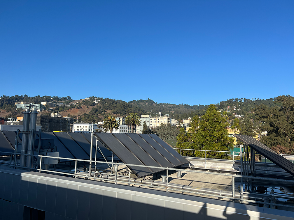
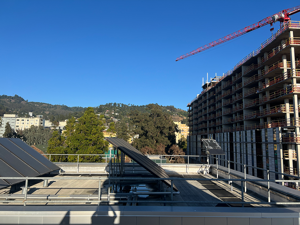
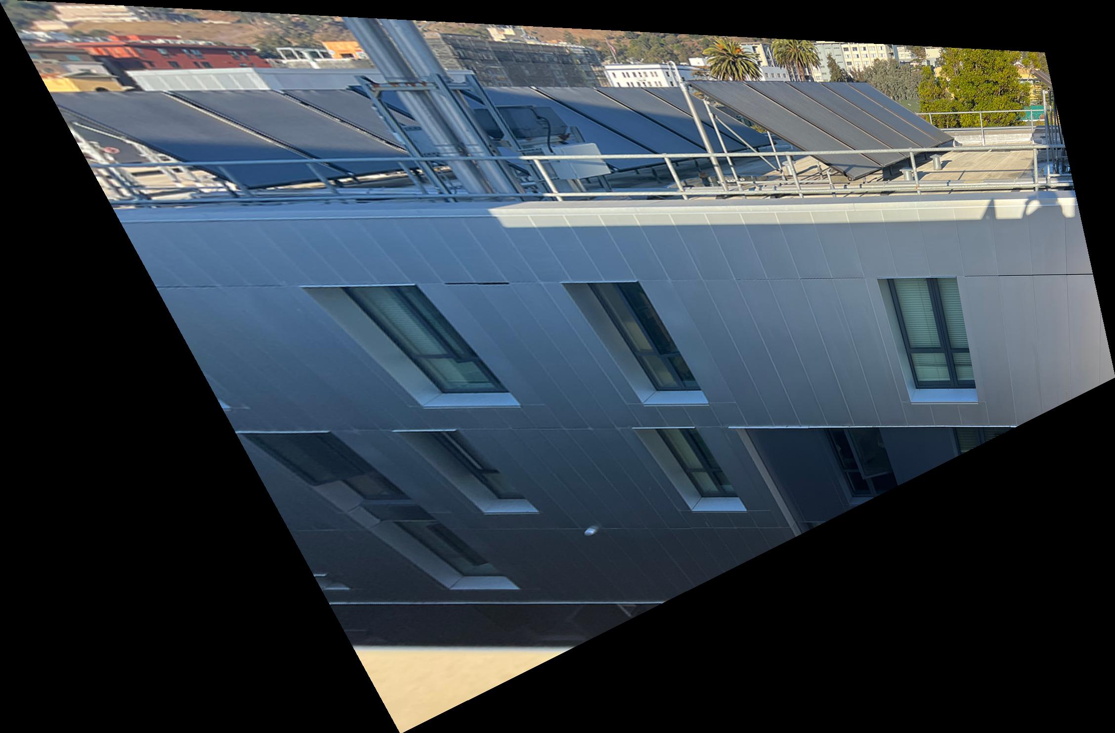
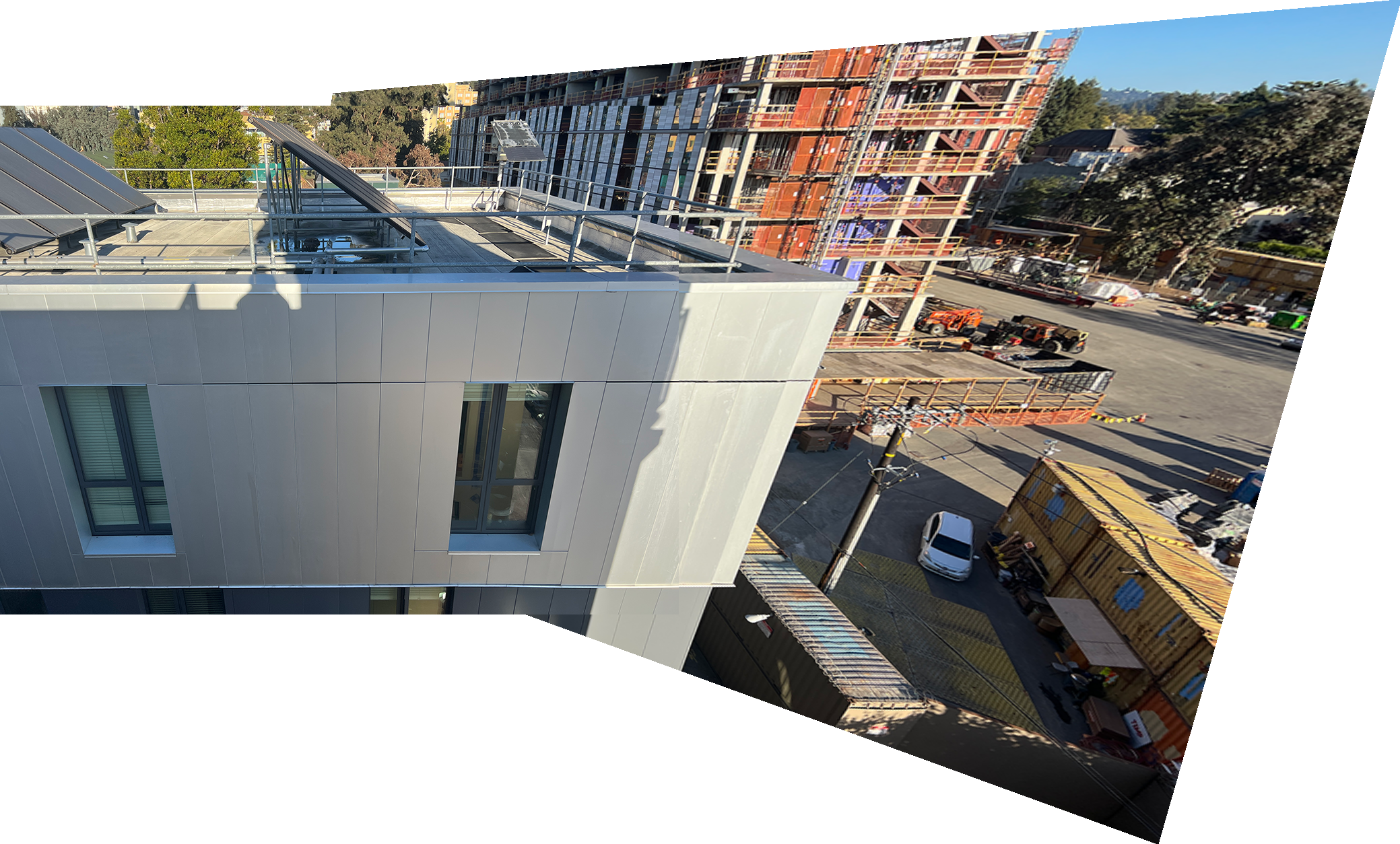
Below are 2 examples of set images that we can warp to form a larger combined image.
Part 2
To combine the images above, we can perform a projective transformation on one of the images such that it will match the other. Because the only change in amera position is rotation, we can compute a homography between 4 chosen points on 2 images that correspond to the same object. In the first example, we will choose the 4 points that maps to the rightmost window of the building.
Using the points
xy1, xy2, xy3, xy4, uv1, uv2, uv3, uv4 = (
    (303.4064, 446.3877),
    (449.93048, 419.11496),
    (447.79144, 660.29144),
    (322.123, 702.5374),
    (689.78, 411.4477),
    (851.77454, 410.35315),
    (802.5195, 661.00684),
    (665.69977, 661.00684)
)
we can obtain the system of equations

which produces the homography matrix
[[ 5.07543229e-01 -9.06493462e-02  4.94054627e+02]
 [-5.71786088e-02  8.91384807e-01 -1.81376979e+01]
 [-5.12480937e-04  8.13734006e-05  1.00000000e+00]]
This will allow us to warp the right image such that the window above will match the one in the center image.
Part 3
With our homography matrix H, we can theoretically directly map the source image to the destination. However, the mapped pixels would not be all integers, which would result in pixels that are not mapped. TO solve this issue, we can use inverse mapping, by first starting with a destination pixel as a vector in the form [u, v, 1]T and multiplying the inverse H-1 to obtain the pixel from the source image that should be mapped to the destination pixel, and use 2 methods for computing the color of the pixel from the source: Nearest Neighbor and Bilinear Interpolation.
To compute the bounds of where to take inverse mapping from, we can transform the coordinates (-0.5, -0.5), (W - 0.5, -0.5), (W, H), and (-0.5, H - 0.5) to provide an upper bound of the transfromed image. We can then round the result to the closest number in ℤ + 0.5, which is equivalent to casting the result to an integer, since we only need the integer coordinates. Below is a comparison of the 2 methods.

From the above, we can see that the Nearest Neighbor method introduces jagged edges due to only sampling from exact pixel values, while the Bilinear method produces a smoother image.
We can also perform image rectification using this tool by transforming a non-rectangular region into a rectangular one. Because we only care about the pixels in the selected region, we can precompute the final dimensions of the rectangle and only perform inverse mapping on the given region. Below are 2 examples of rectifying an image:
Part 4
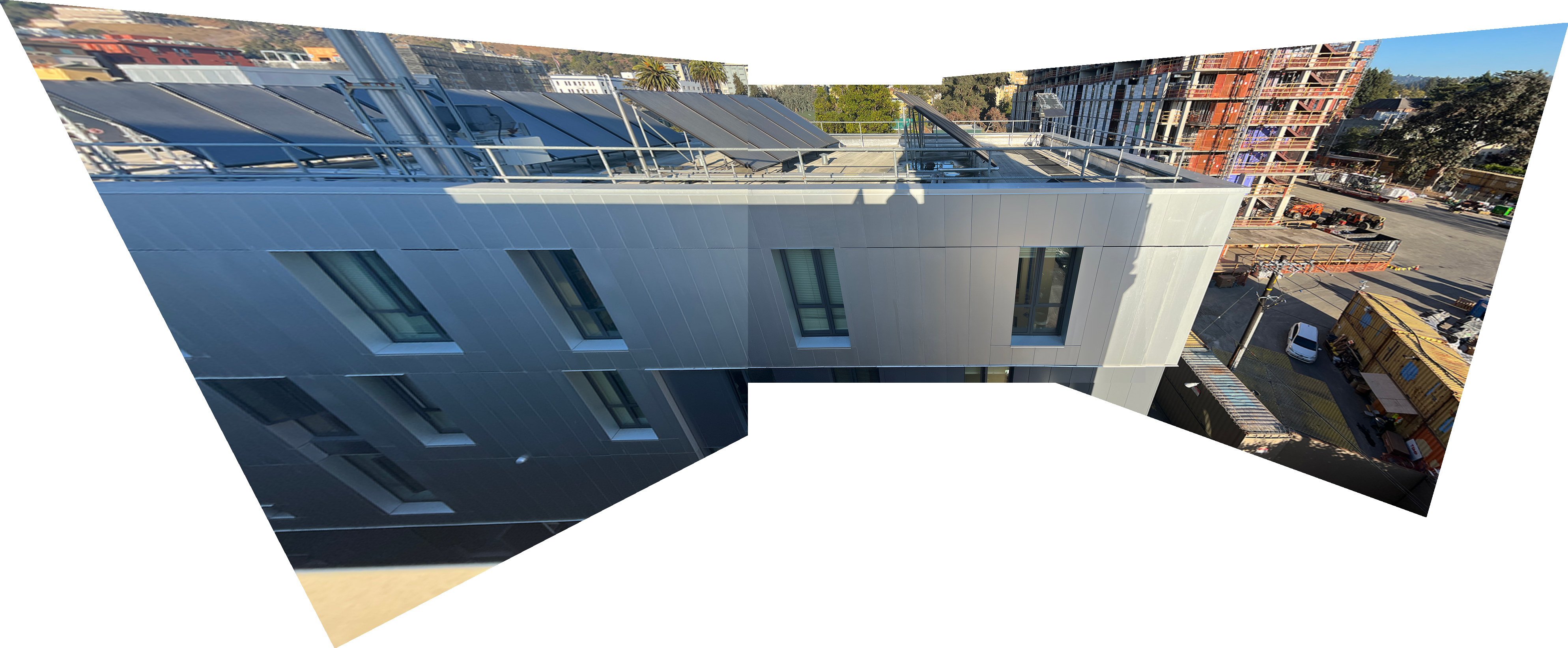
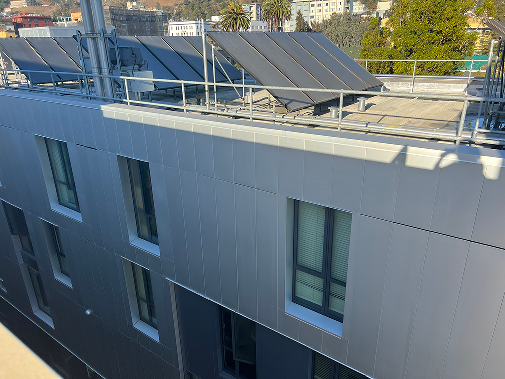
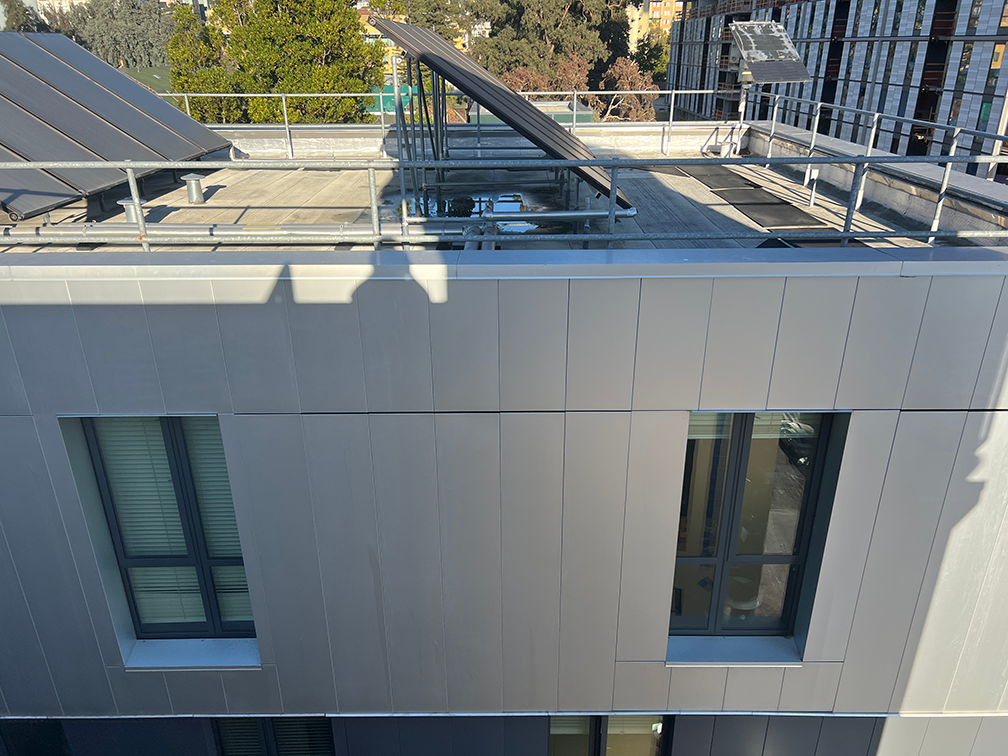
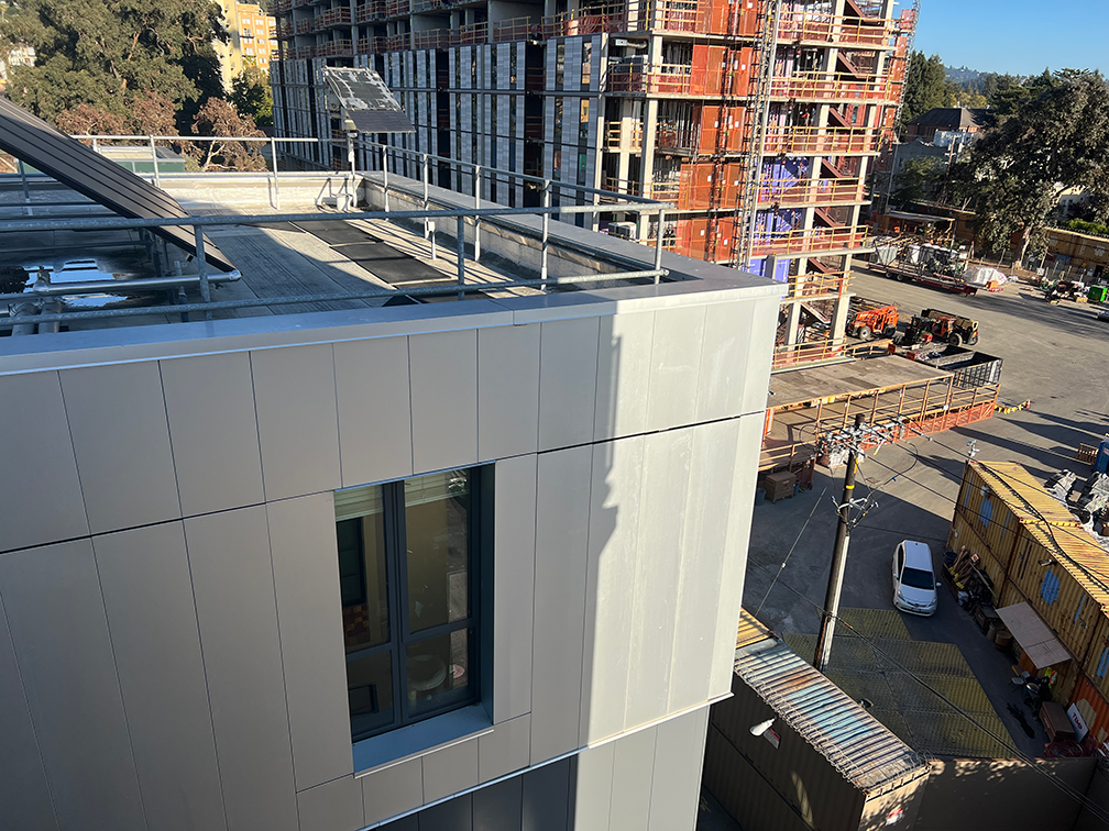
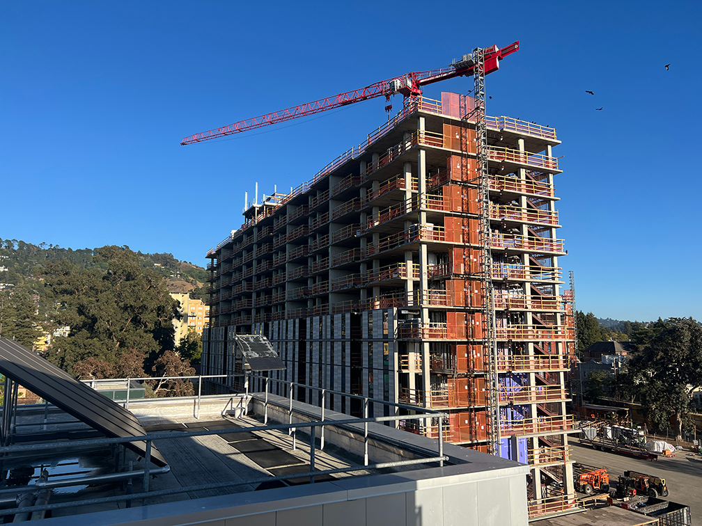
With these tools, we can create a panoramic mosaic of multiple images. Take 3 images below:
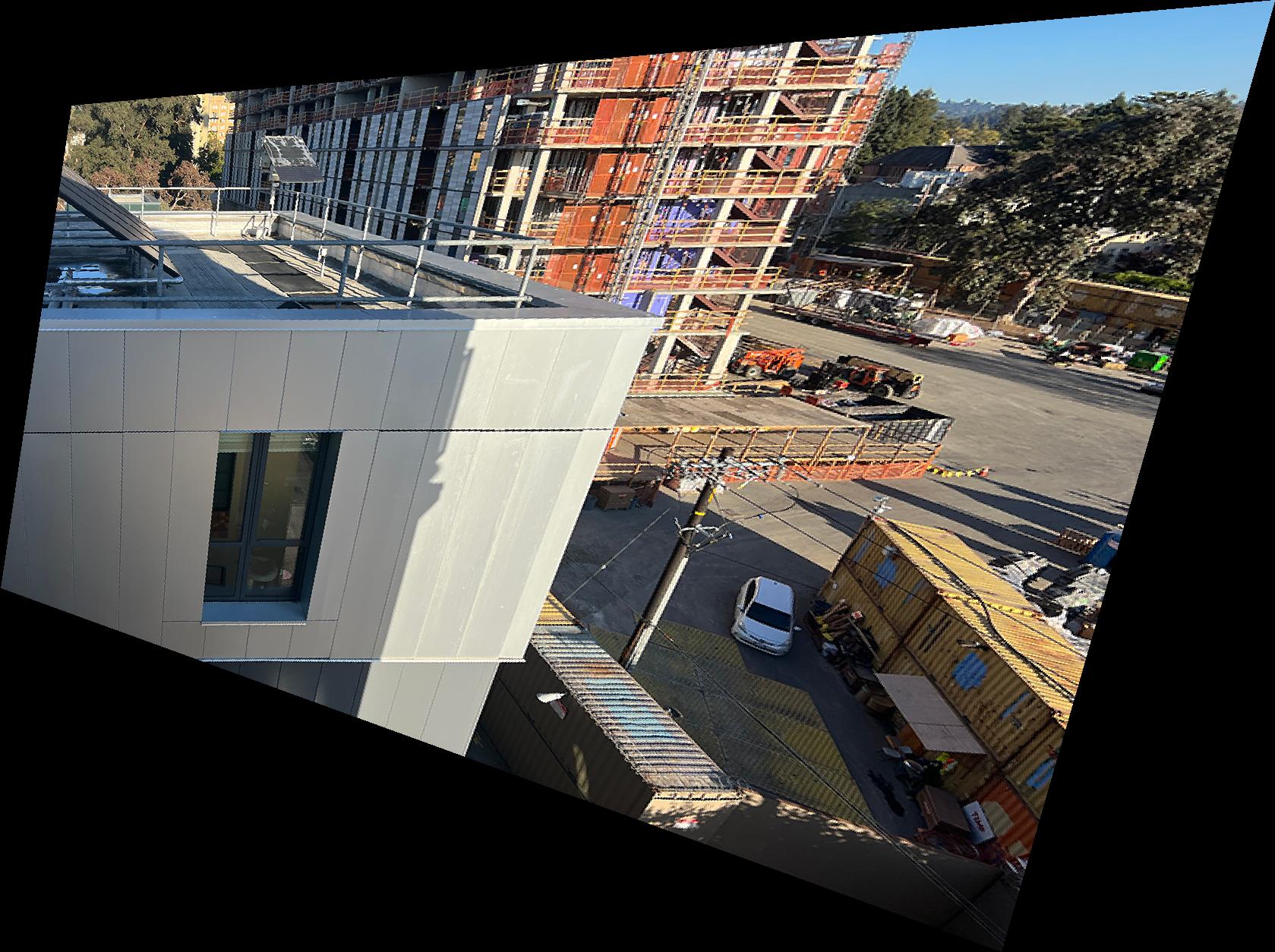
We can first compute the homography of the right image and warp & stitch it with the center image. Once this is done, we will compute the pixel offests of the stitched center-right image with the original center image, so that the center image pixels matches with the center image the homography of the left and center image is computed with.
Because we have already warped the left image, we can simply stitch it with the stitched center-right image, creating the following 3-image mosaic: