Part 1.1: Convolutions from Scratch
Using the definition of convolution:
for result_i in range(result.shape[0]):
    for result_j in range(result.shape[1]):
        total = 0
        for i in range(ffker.shape[0]):
            for j in range(ffker.shape[1]):
                total += img[result_i + i, result_j + j] * ffker[i, j]
        result[result_i, result_j] = total
return result
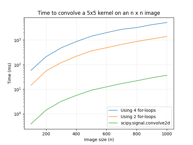
where ffker is the xy-flipped kernel and result is the output 2D array, we can slightly speed up the computation by replacing the 2 inner for-loops with result[result_i, result_j] = np.dot(img_flat, ffker.flatten()), where img_flat is the flattened 1D array of the current patch of img based on the position of the kernel. Although this optimization produces a noticeable speed-up compared to using 4 for-loops, the fastest way is still to use scipy.signal.convolve2d. Below is a timing comparison of the 3 methods above using a 5x5 kernel:
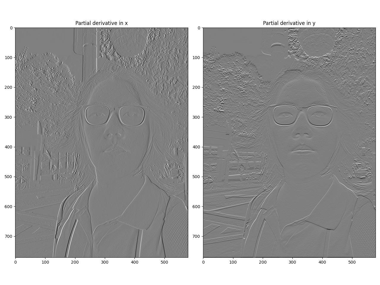
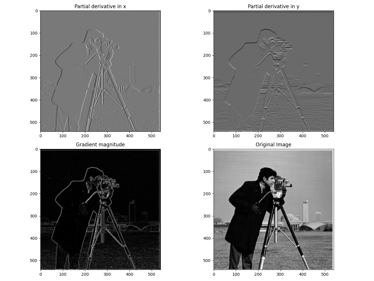
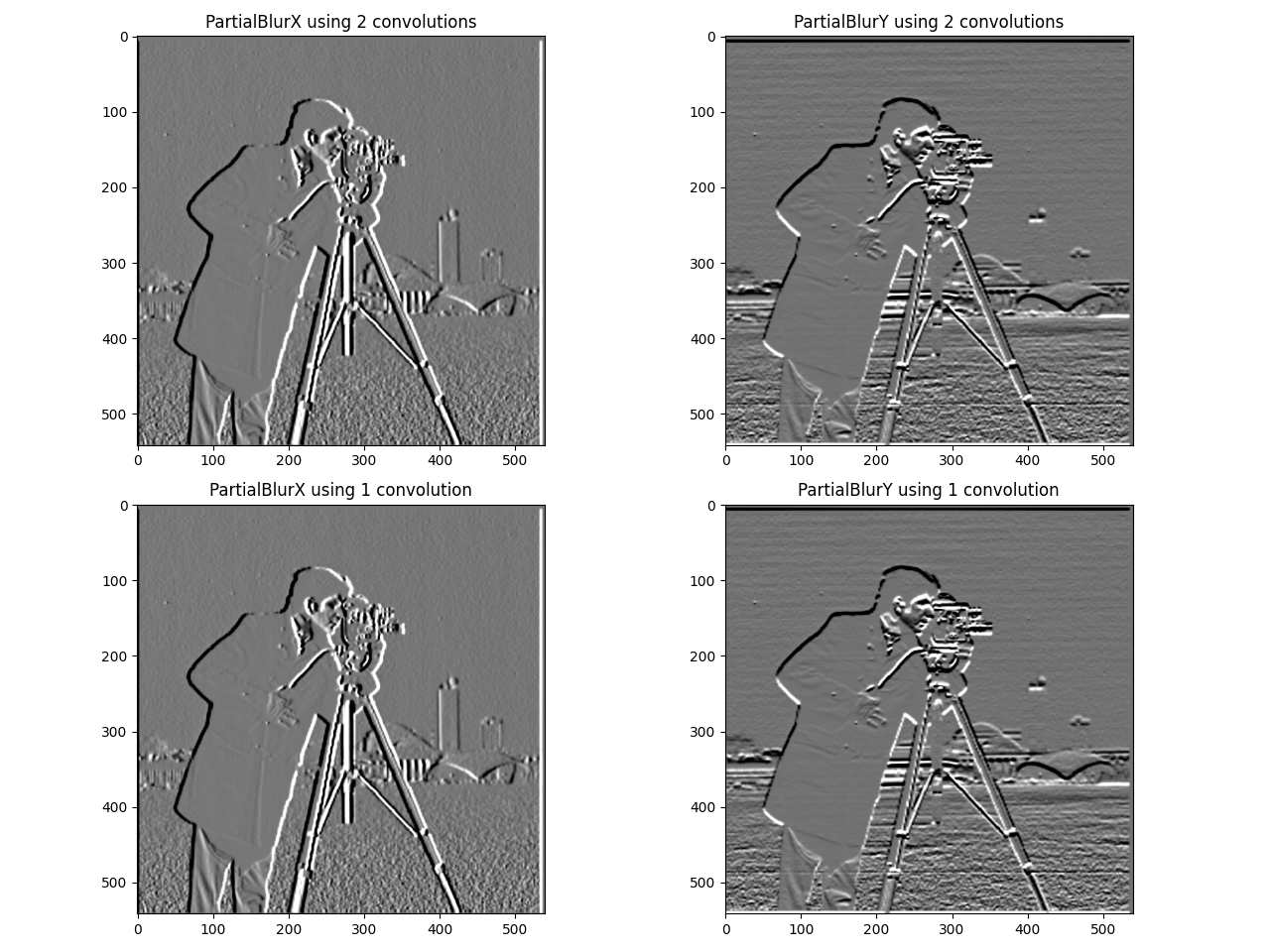
To demonstrate an application of convolution, we can convolve an image with the box filter, a kernel with entries that sum to 1 that contains only 1 unique value. We can also convolve with the difference operators 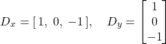 for edge detection. Each kernel computes the difference in the x- or y-direction, so edges where the brightness of the pixel changes significantly will show up as white and black pixels on the output. Using
 box_9x9 = J9 / 92 as the box filter, we get the following results:
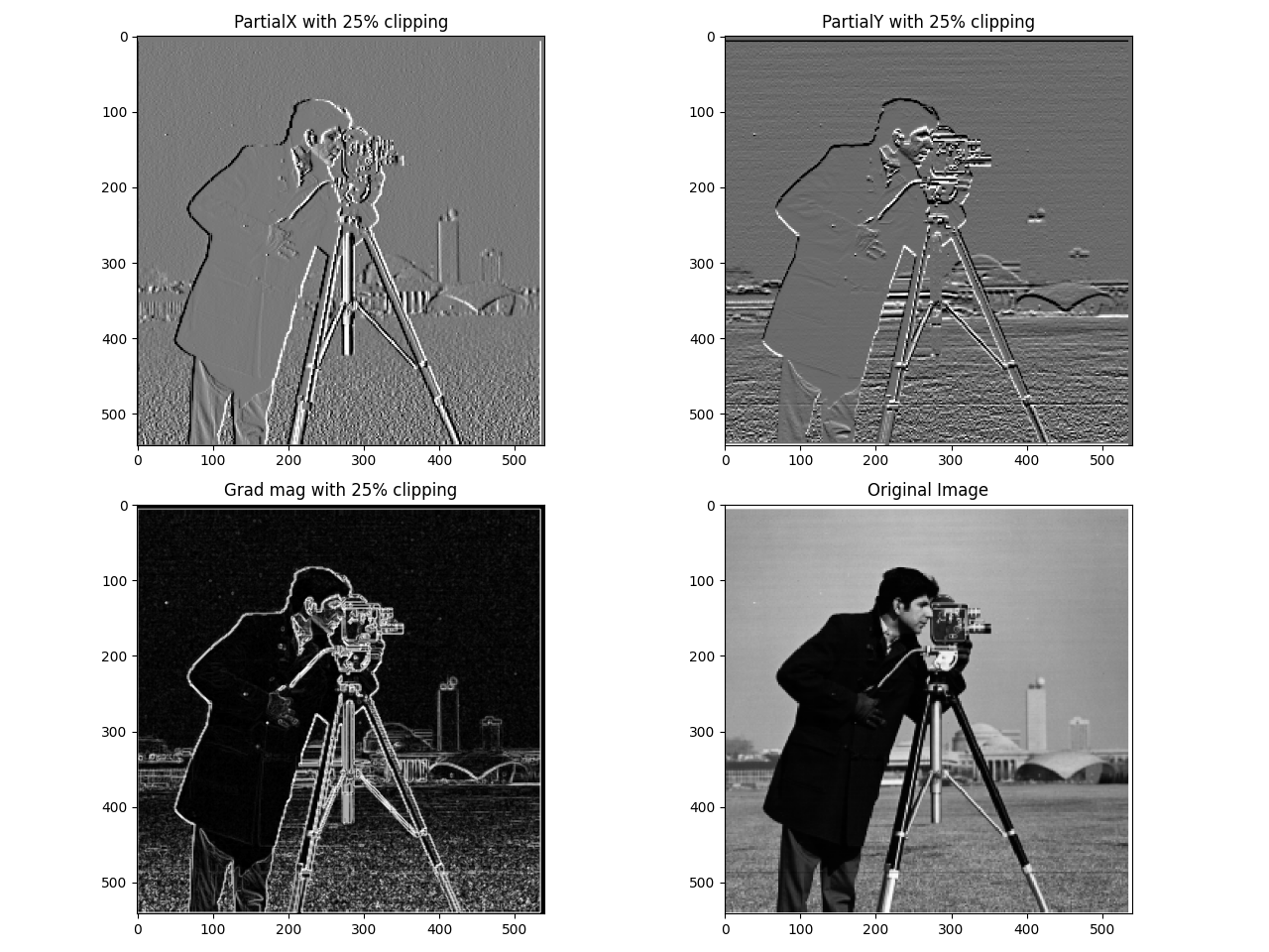
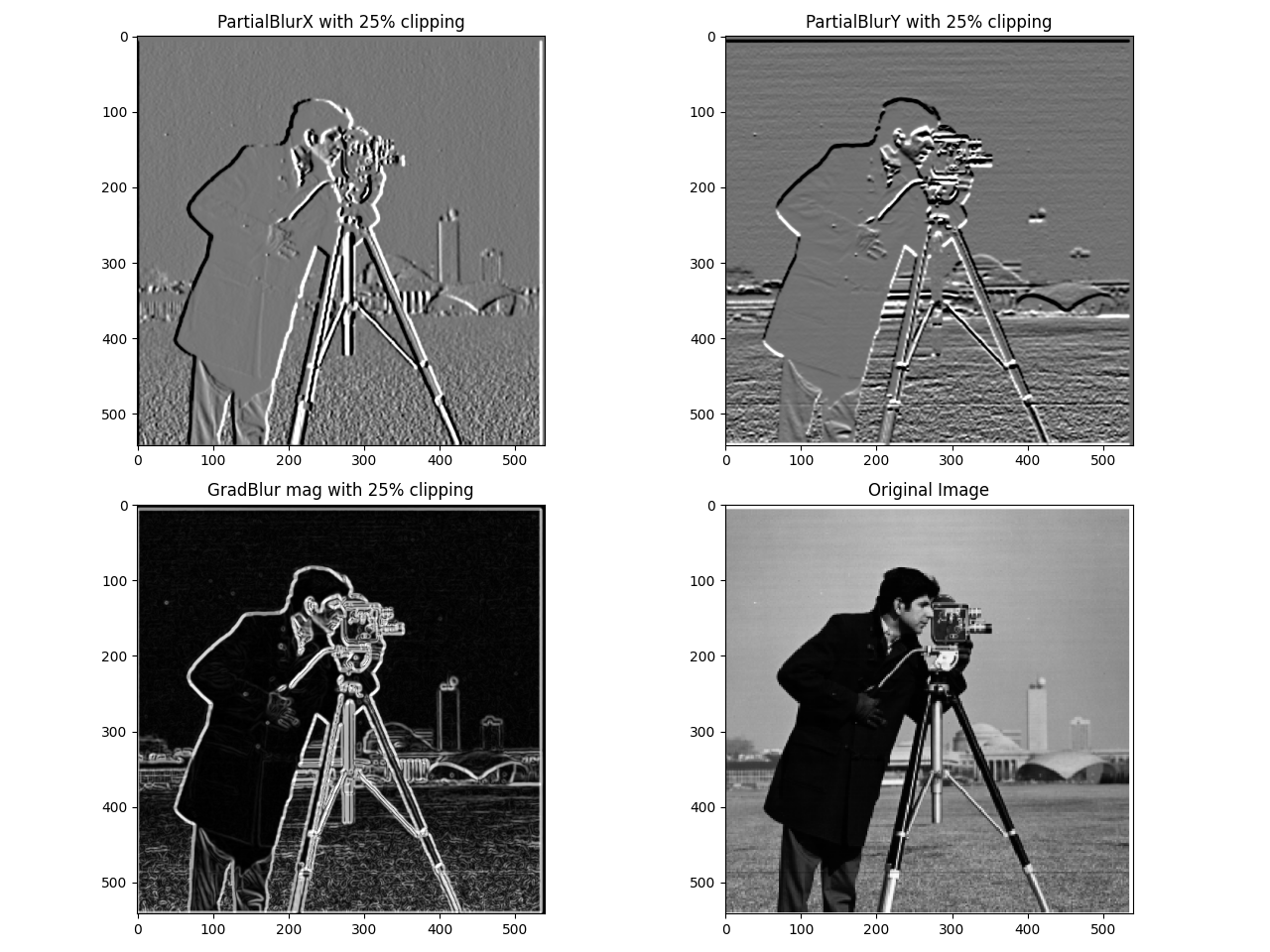
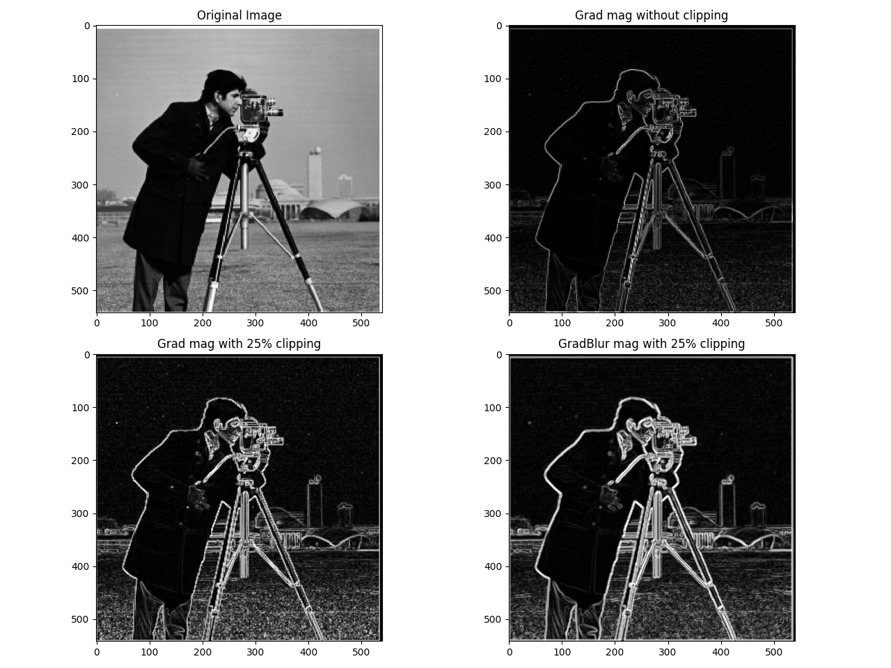
For convolving with Dx and Dy, we have:
To handle boundries, we can set all of the padding pixels to 0, similar to the following:
if mode == 'valid':
    return convolve(img, ker, naive)
elif mode == 'same':
    pad_ht = (ker.shape[0] - 1) // 2
    pad_wl = (ker.shape[1] - 1) // 2
    img_padded = np.zeros((img.shape[0] + ker.shape[0] - 1, img.shape[1] + ker.shape[1] - 1))
    img_padded[pad_ht:pad_ht + img.shape[0], pad_wl:pad_wl + img.shape[1]] = img
    return convolve(img_padded, ker, naive)
elif mode == 'full':
    pad_h = ker.shape[0] - 1
    pad_w = ker.shape[1] - 1
    img_fpadded = np.zeros((img.shape[0] + 2 * pad_h, img.shape[1] + 2 * pad_w))
    img_fpadded[pad_h:pad_h + img.shape[0], pad_w:pad_w + img.shape[1]] = img
    return convolve(img_fpadded, ker, naive)
else:
    raise ValueError('Unsupported mode: ' + str(mode) + '. Must be one of \'valid\', \'same\', or \'full\'.')
A zero-valued pixel, however, is equivalent to a black colored pixel on the image. This means the function would introduce a dark edge if one wants to have the image be the same size after convolving, which is visible above. To prevent this scenario, the safest way is to let the first row/column be the first padding row/column on the top left side, and perform the same with the last row/column on the bottom right side. This process can also be carried out for the 2nd/2nd-to-last row/column, and so on. Compared to other approaches like 'wrap', this method ensures that there won't be significant artifacts by ensuring the padded pixels come from the closest pixels in the image. To implement this method, we can set the boundary variable to 'symm' in convolve2d. In comparison, the zero-padding mode is the same as the default mode in convolve2d, which shows how convolve2d has more functionalities than the naive implementation.


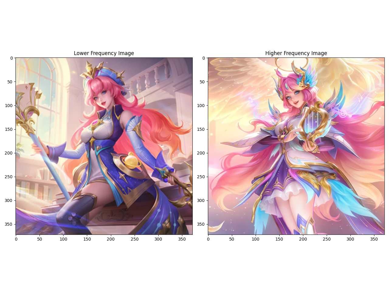
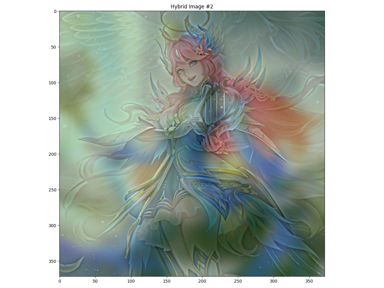
![[1]](https://mobile-legends.fandom.com/wiki/Odette?file=Odette_%28Wisdom_of_the_Stars%29.jpg)
![[2]](https://mobile-legends.fandom.com/wiki/Floryn?file=Floryn_%28Melody_of_Light%29.jpg)
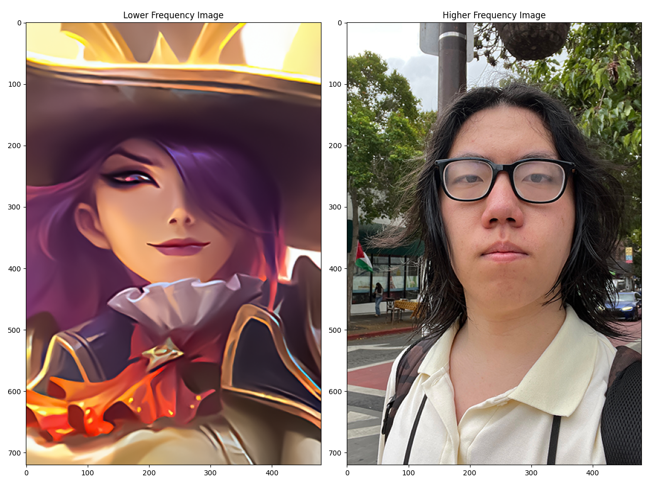
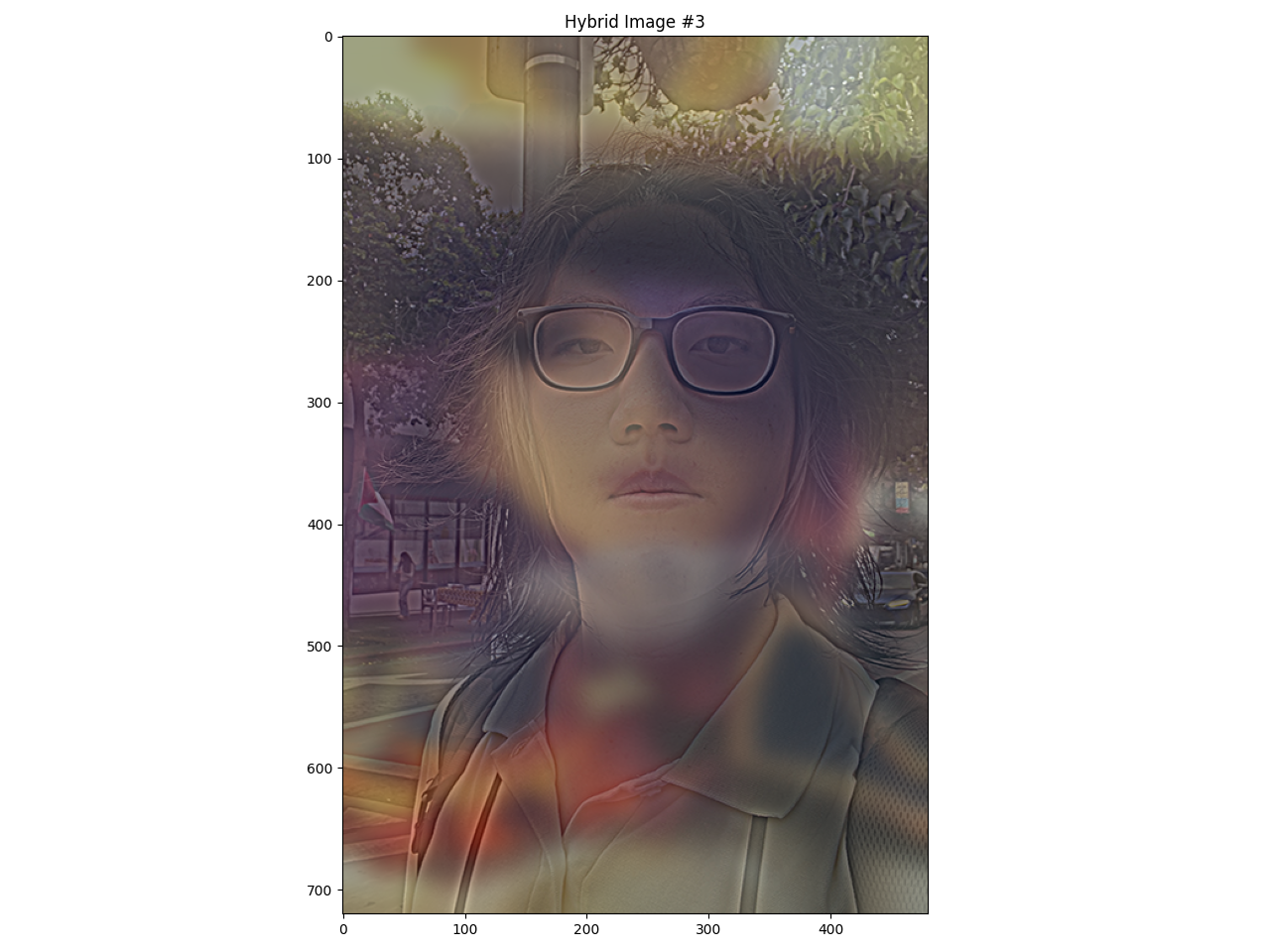
![[3]](https://mobile-legends.fandom.com/wiki/Lesley?file=Lesley_%28Angelic_Agent%29.jpg)