
by Daniel Cheng | September 12, 2025
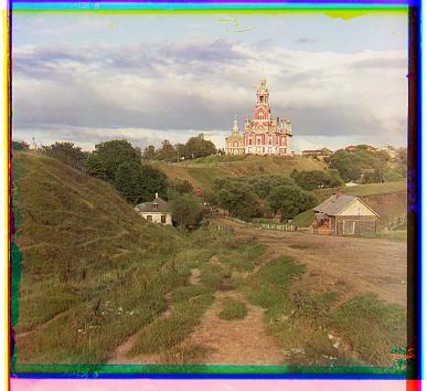
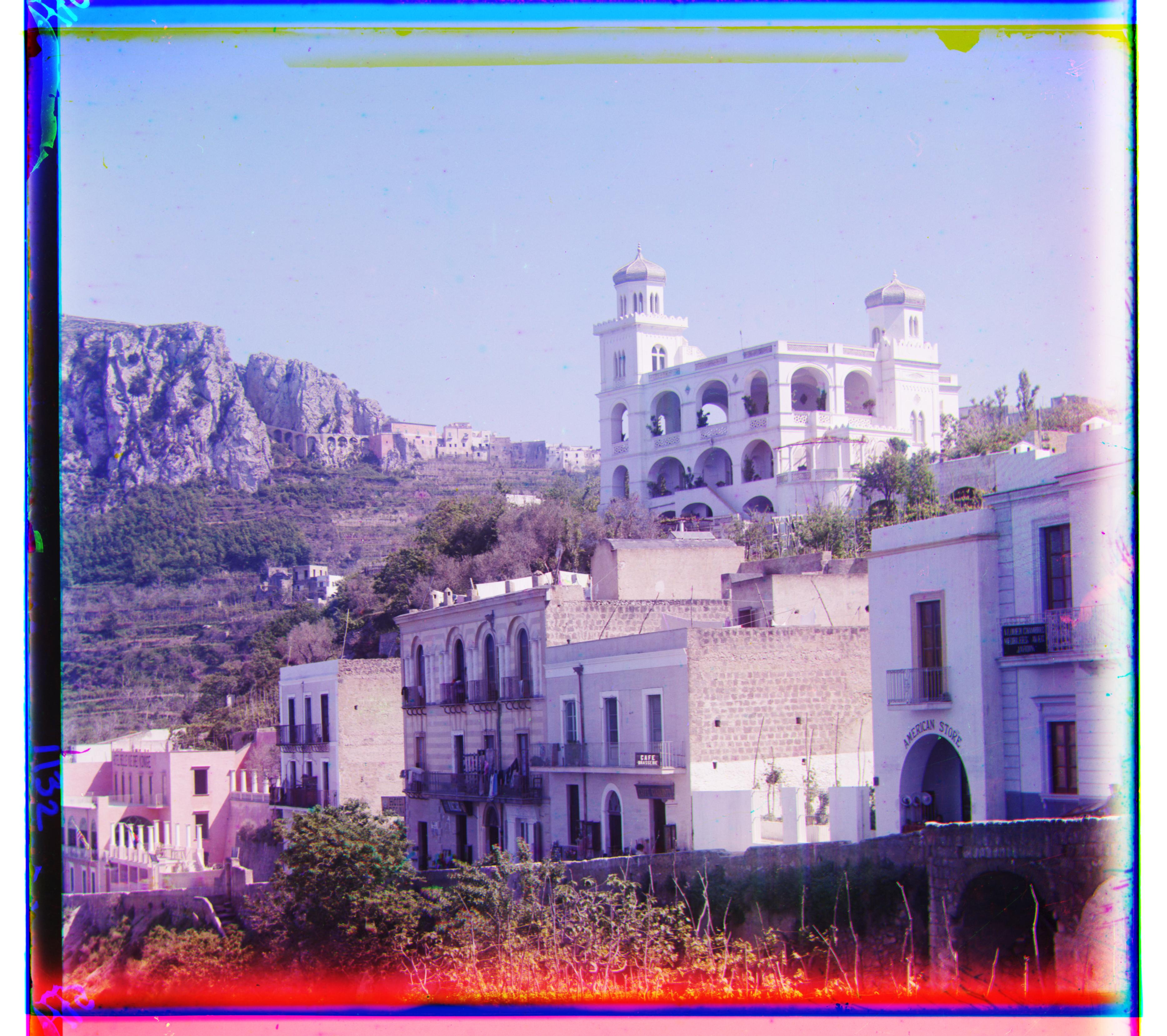
The Prokudin-Gorskii photo collection consists of 3 glass plate images, each taken in grayscale with a blue, green, and red filter (ordered from top to bottom). To obtain a colorized version of the original image, we can align the images and use the pixel brightness (normalized to [0, 255]) from each image as the value of its respective color channel. This project aims to perform the aligning and compositing process automatically, given any image containing the 3 glass plates in BGR order.
To begin the alignment process, we need a function that can compute a similarity score between 2 images. Motivated by the fact that given a + b = c, ab attains its highest value at a = b = c/2, we can use the normalized cross-correlation

for 2 vectors x and y. After normalizing each image with the L2 norm, the dot product will ensure that the score will be the highest when the features of both images are the most similar. Since grayscale images are represented by 2d arrays, we can first flatten the 2 images we want to compare, before using them as the input vectors. A caveat of this method is that both images should be the same size. However, we can approximate the crop dimensions for just the blue and red plates and find the best displacements with respect to the green plate. The final step would require us to find the intersection of 3 rectangles, which is illustrated below:
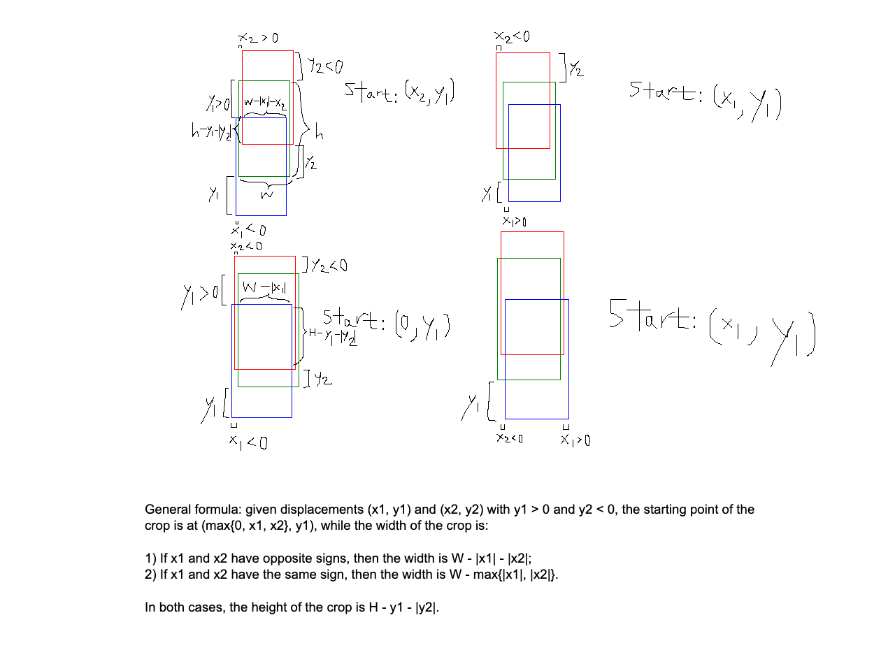
To find the best shift, the simplest way is to compute the NCC for every possible shift within the full image. However, not only is this inefficient, but the best shift would also just be (0, 0) for any image, since the crop would just be a copy of the original crop. To solve this issue, we need to limit how much the height can shift when aligning.
Define W and H to be the width and height of the full image, and assume, for approximations, that each plate takes up exactly a third of the full image. Considering only the top/blue plate, we can start by setting the upper limit for the top edge to be (0 + H/3) / 2 = H/6, and the bottom edge to be (2H / 3 + H) / 2 = 5H / 6. This means the top edge should be at least shifted down by H/6 - 0 = H/6, and the bottom edge by 5H / 6 - H/3 = H/2. Therefore, a good place to start is a displacement of (0, (H/6 + H/2) / 2) = (0, H/3) with a search range of [-H/6, H/6]. For the bottom/red plate, the equivalent displacement is just (0, -H/3) with the same search range. Any shifts that bring the crop outside the original image will be ignored.
Using a starting crop of {(W/16, H/16), R(W - W/16, H/3 - H/16)} for the blue plate and {(W/16, 2H / 3 + H/16), R(W - W/16, H - H/16)} for the red plate, where the tuples are the upper left and lower right corner pixels in (x, y) coordinates, we can obtain the following best shifts:


Unfortunately, because each crop has a height of (7W / 8) × (5H / 24), the total number of NCC computations for each alignment is ((W - 7W / 8) + 1) × ((H/3 - 5H / 24) + 1) = (W / 8 + 1) × (H / 8 + 1) = O(HW). Since each NCC computation requires O(HW) operations, aligning an image of dimensions W × 3W takes O(W2) time using the naive search above. Because the .tif files are about 9 times bigger than the .jpg files in both dimensions, performing the same search on these files will take more than 6500x more times longer to compute. Even if we don't crop horizontally at all, it would still have a complexity of O(W3) and require more than 93 ≈ 720x more time on .tif files. A more efficient method is required.
Instead of searching over the entire image, we can scale down the image, find the best shift at a much smaller size, and scale the result back to its original size. Once the most accurate displacement (xlowest, ylowest) is calculated for the lowest-sized image, we can perform another search at the image 2x the size. Only this time, we start at (2xlowest, 2ylowest), and only search over a window of [-2, 2] for pixel corrections. Once the best displacement at the layer below the lowest scale is computed, we can multiply the result again by 2 and pass it to the image in the next layer below. The limited window is used because each downscaled coordinate could have only come from a total of 4 different coordinates, so the best coordinate on the higher scale is limited to [-1, 1] of the interpolated coordinate. An additional pixel in the search range is used to further reduce the effect of noise on the best placement at the lowest scale. To further optimize this approach without storing all downscale images at once, we can modify the best displacement function to have a recursive call.

Now, we will only calculate the best displacement if the given width is below a certain threshold. For images above this threshold, we can first downscale the image by 2x, pass it back to the function, and the returned shifts are scaled up by 2x to return the best shifts on the input image. This means that the best shifts in the base case (xlowest, ylowest) will be scaled up and used in the previous recursive call, which is the scaled image 1 call above. This will continue until we return to the top-level call, and at that point, the returned shifts will be within 1 or 2 pixels of the best overall displacement. The last thing to keep in mind is to downscale the cropping box as well, which is simple to do since it is computed on the full image, and one can simply divide its coordinates by 2 for each recursive call. In practice, setting Wmin = 72 gives the best tradeoff between the search size and the number of rescales. With these optimizations in place, the computing time is now much faster:


Even for small images, the pyramid method achieved a speedup of over 100x due to a reduction in both size and number of NCC computations, while for large images, the computation time is still faster than what naive search takes on a single small image. More concretely, because the image is downscaled by 2x at each layer of the pyramid, the total image area is less than 1 + (1/2)2 + (1/4)2 + (1/8)2 + ... = 1 + 1/4 + 1/16 + 1/64 + ... < 4/3 of the original. Since the search at the lowest scale is limited to W ≤ 72, the total time complexity is only 4(3W)W / 3 + smaller terms = O(W2), which matches with the actual factor of ~100 between the time it takes to align .jpg and .tif files.
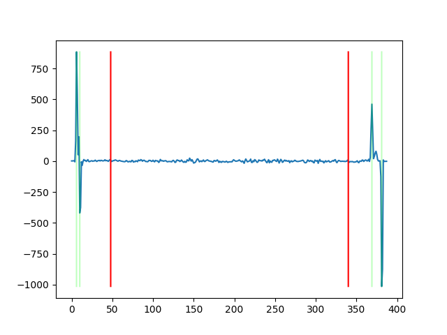
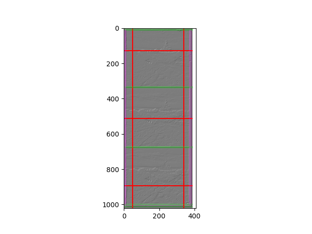
Although having a fixed cropping dimension worked for aligning the images, because the final result is simply the intersection of the translations, artifacts from the border still remain. Is there a way to automatically crop the borders? The answer is yes. We can start by convolving the sobel operator


with the base image, and add the results together. This will produce a composite of the detected edges along the x- and y-axis. The next step is to reconstruct the borders of each plate from the image. Because Sobel is distance-invariant, we can convolve the kernel on only the valid patches, resulting in the new image having dimensions (W - 1) × (H - 1).
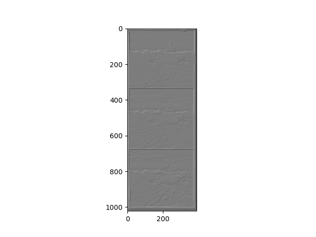
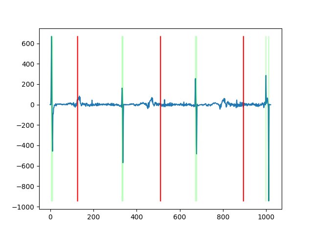
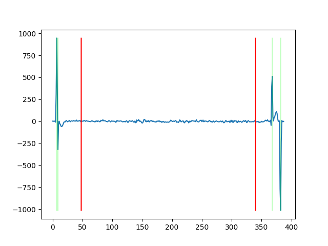
Now, we can take the average of each row, and those with the lowest and highest values will be the edges. By splitting the resulting array into 4 subarrays [0 : H/8], [H/8 : H/2], [H/2 : 7H / 8], and [H/8 : H], we can find the argmax and argmin in each subarray, which will be used as the horizontal borders of each plate image.
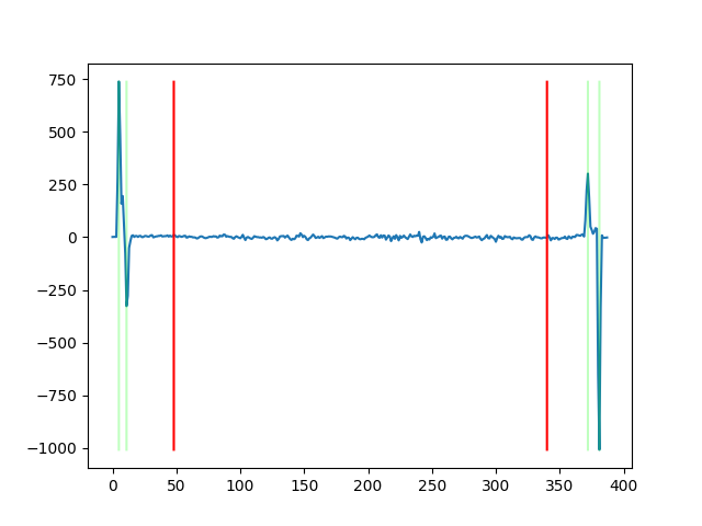
The vertical borders can be computed using a similar strategy, except that we need to split the column averages into 3 subsections based on the values found in the previous part. This will ensure that we are able to find the vertical edges of each plate image. Although the center/green plate is not used in the alignment process, its borders will be needed to compute the final crop of the composited image.
Once the best displacements for the blue and red plates are found, the final step is to find a way to merge the 3 crops, which can be done in the following steps: First, find the intersection of all shifted crops. Second, shift them back to their starting position using the inverse of the displacement. Finally, shift the pixels from the starting positions back to the center using the best displacement, and combine the 3 crops into their respective RGB channels. As a failsafe for bad starting crops, the normal overlap method (discussed in the NCC & Preprocessing section) will be used instead. At the cost of doubling the runtime due to convolution, the images are now much cleaner:

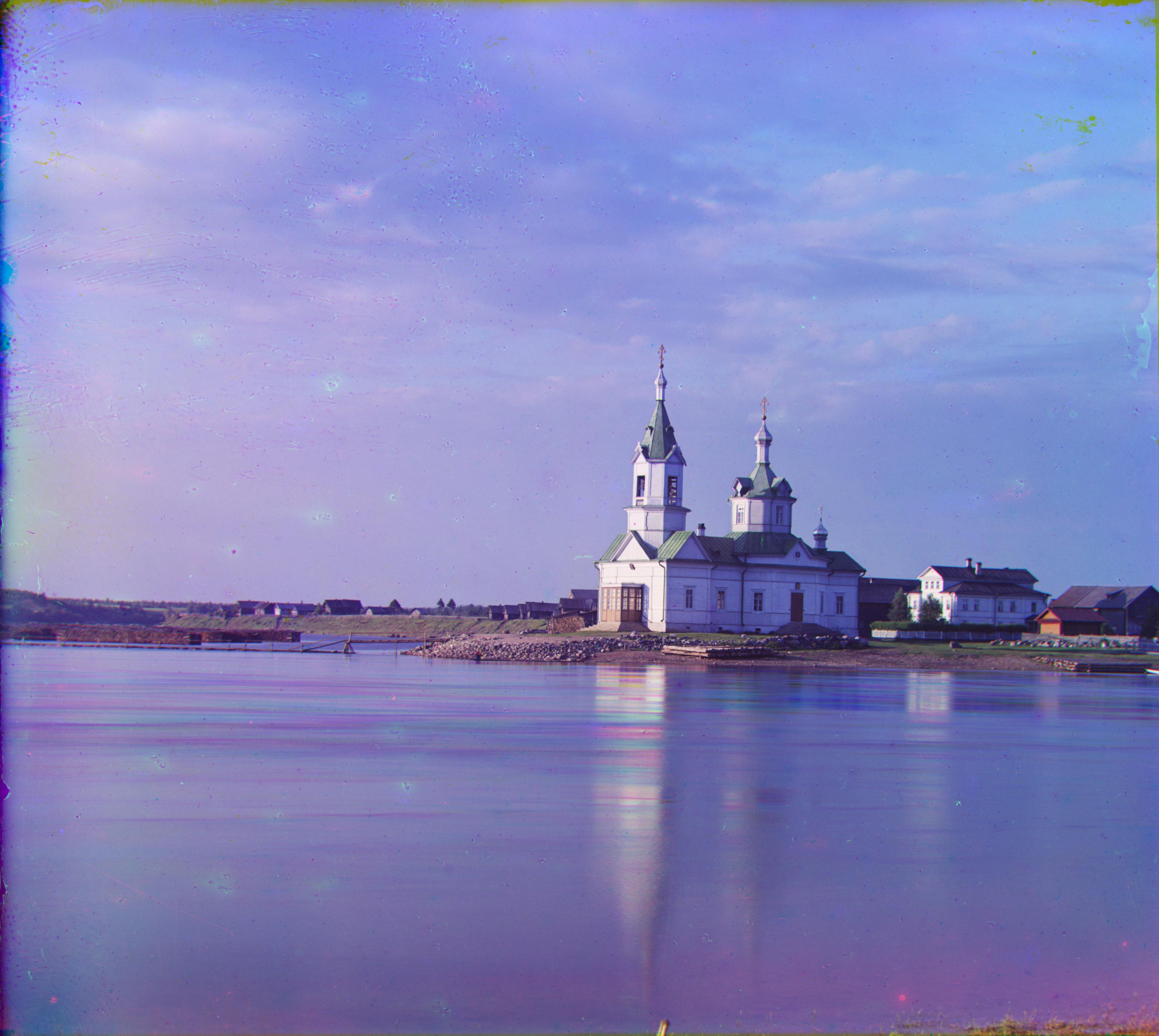
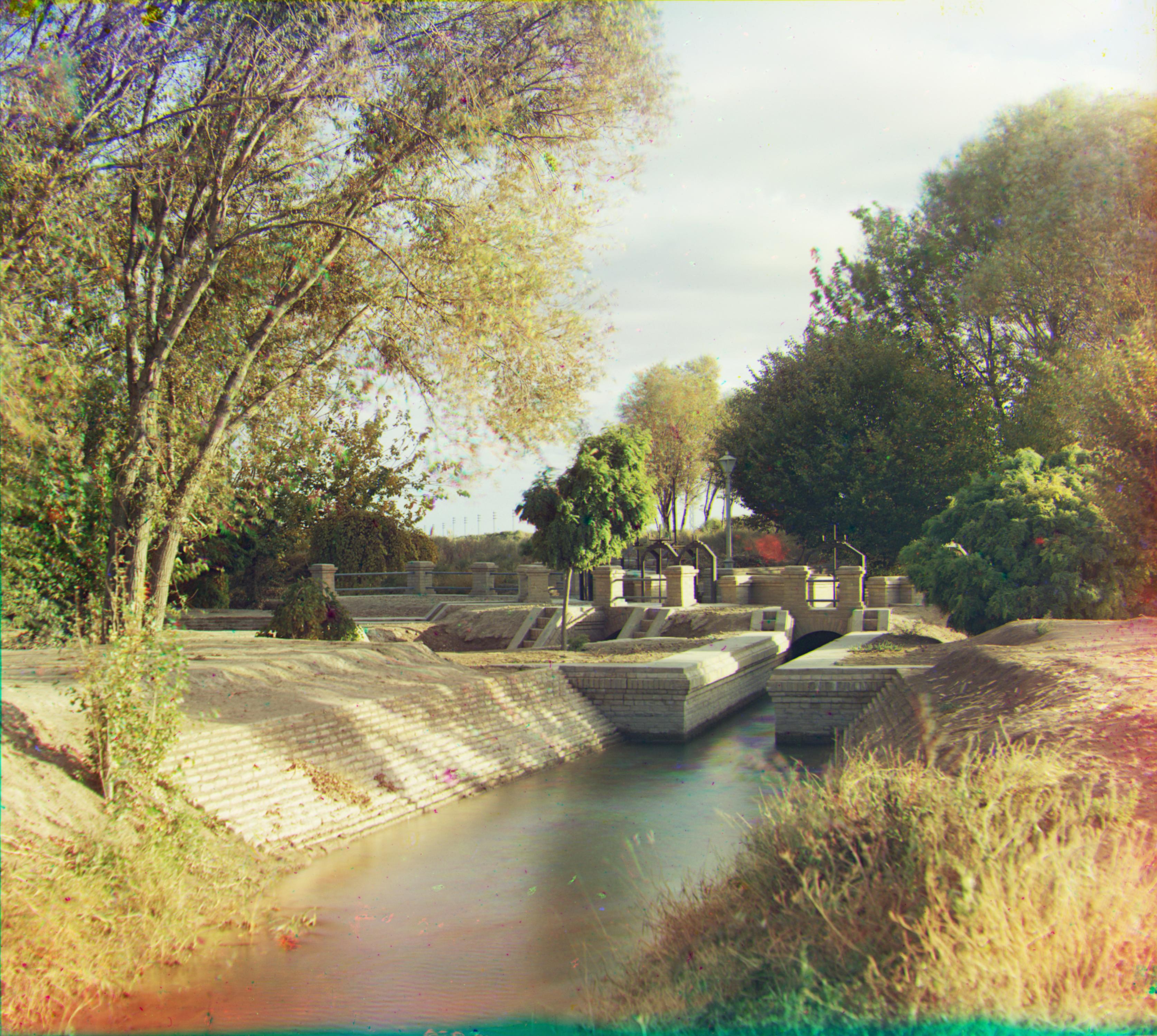
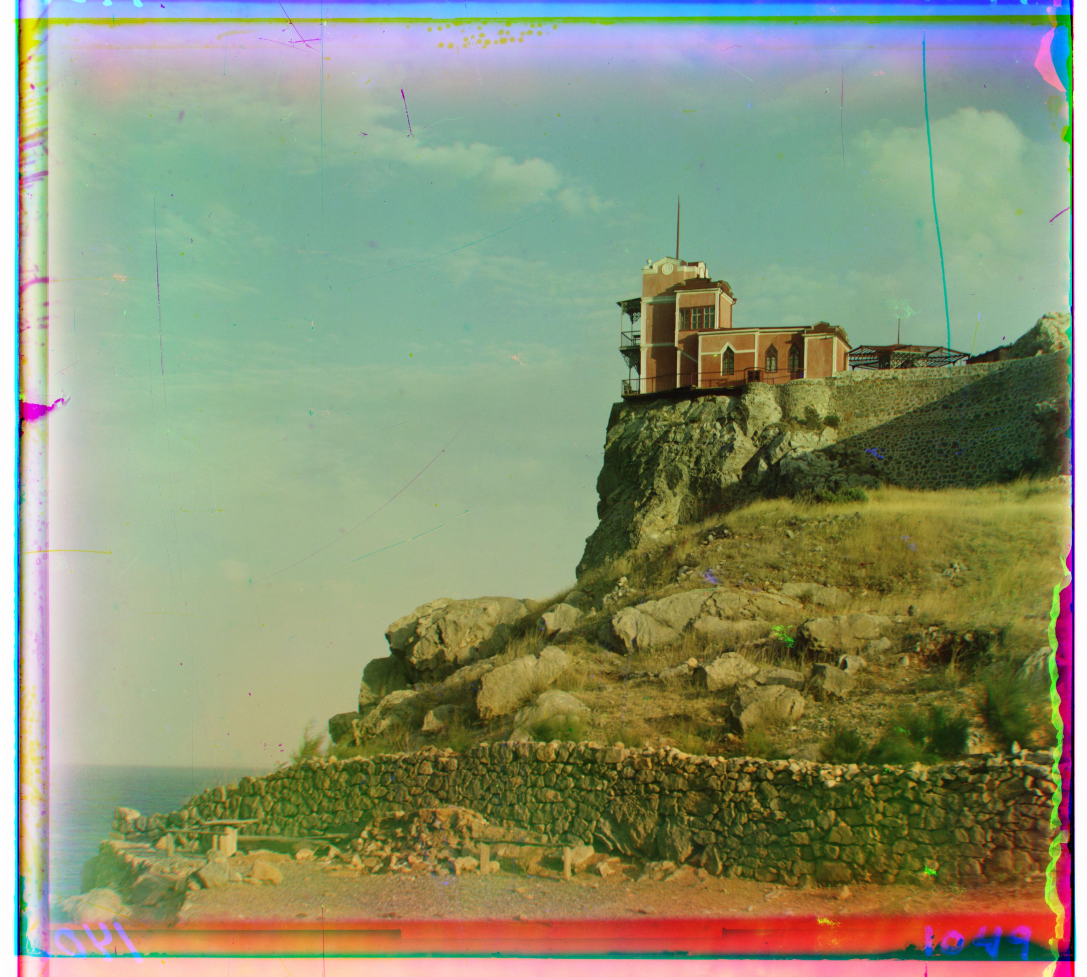
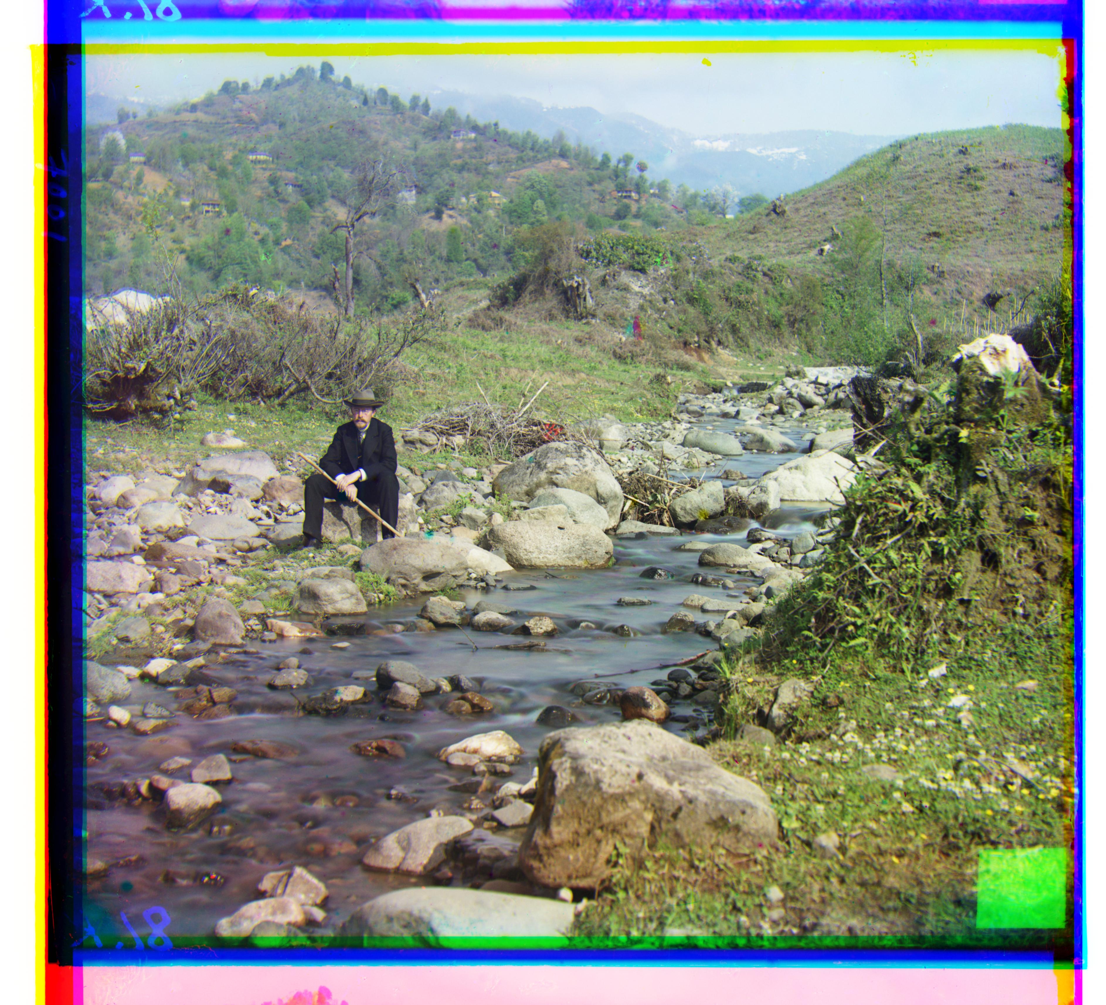
The title image was computed with a best shift of B(-23, 3159), R(17, -3152) in 6.26317s.